Data
When looking at an ordinary tennis match, there are many different sounds that can be heard, but only some of which are relevant to the scoring of a tennis match. In particular, those sounds are a ball hitting a racket, the ball hitting the net, and a line umpire calling a ball out. The rest of the sounds in a tennis match (crowd cheering, chair umpire announcing score, commentators talking on the television broadcast, etc.) don’t have any effect on the scoring of the game. To reach our goal of being able to score a tennis match, we have to identify the characteristics of the important and not important sounds.
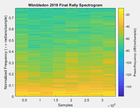
To do this, we employed MATLAB’s FFT and Spectrogram functions to help quantify and identify characteristics of audio clips of tennis matches in the frequency domain. Each audio clip was pulled from a Youtube video of a broadcasted tennis match and cut up to only focus on one of two events: a rally between the two players, with each player having multiple hits, and the applause from the crowd immediately after the rally had finished. Each of these clips were plotted in the time-domain and in the frequency-domain using the FFT and Spectrogram functions. An example of one of these audio clips of a rally is shown below in Figures A-C.
Figures A-C: Time-domain plot of audio clip, FFT, and Spectrogram plot (L to R) of rally from audio clip of 2019 Wimbledon final
It was concluded that including multiple hits in the same Spectrogram and FFT plot didn’t paint a clear picture where we could learn about the frequency-domain characteristics of a ball getting hit by a racket. So in our next iteration of analysis, we shrunk down the time scale of the audio clip to only include one singular hit of the ball. And in an attempt to visualize the data we were plotting, we plotted each hit in time-domain, Spectrogram pairs for quick and easy comparison between the two plots. Shown below in Figures D & E are examples of these pairs of plots.
Figures D & E: Shortened time scale time-domain and Spectrogram plot pairs of a ball getting hit by a racket. Taken from rally at 2019 US Open
Our initial predictions for these plots were the clips of a ball getting hit were going to be very similar to delta functions, they would have a relatively high amplitude over a very short period of time. This prediction would lead us to infer that this audio event would have a large component of its auditory power at higher frequencies, which would be illustrated on the spectrograms on Figures D & E. Our prediction of there being a very short time period did turn out to be correct as most of the individual ball hit clips we looked at lasted less than 2 hundredths of a second. But our prediction of the ball getting hit being a high-frequency sound wasn’t completely accurate. From inspection of the spectrograms, the majority of the sound’s power is located at low frequencies, with the high-frequency components having very little power by comparison. This is something we predicted would be the main characteristic of the noise immediately after the rally, but due to the complex nature of the racket & tennis ball collision, that characteristic is also prevalent in the audio clips of rallies between the two players.
The other necessity for our filter to successfully identify these ball hits was to characterize the noises that need to be filtered out, aka the ‘Noise’. The same method used to create the plots in Figures D & E was employed to create pairs of plots. The resulting plots are shown below in Figures F & G.
Figures F & G: Time-domain and Spectrogram plot pairs of the noise that occurs immediately after a rally finished. Taken from 2019 US Open
As mentioned above, our prediction for when we plotted the noise clips in the frequency-domain plots was they would have the majority of their power located at lower frequencies and hardly have any components at higher frequencies. And while the shape of the spectrogram plot is very different from the spectrogram of the rally clips, the underlying data is surprisingly similar. Both the rally and applause clips are mainly low-frequency noises, with the rally clips having marginally higher power at higher frequencies.
Our initial plan was to use a high-pass filter to eliminate the low frequency noise from the crowd, but after analyzing individual clips of rallies between the two players and clips of the crowd applauding after the rally had finished, we came to the conclusion that directly applying a filter to an audio clip of a full match would not produce the desired result. Due to the complex nature of the sound when a tennis ball gets hit, applying a high-pass filter to highlight the instances in an audio clip where a ball gets hit would actually eliminate those instances. This information would prove invaluable in creating our own custom filter to identify ball hits during a match.