November 17, 2020

​
 

Table of Contents

​

I. Plots and Data

II. Challenges

III. Next Steps

IV. Acquired Knowledge

 

Plots and Data

Original plots

​

 

 

 

 

 

 

 

​

​

​

​

These are the original two plots that we had for our initial submission, with the audio clip of a ‘rally’ plotted generically on the left, and a graph of that signal’s spectrogram on the right.  The purpose of these plots was to isolate the spikes of the tennis ball hitting the racket and draw some conclusions about it in the plots of the spectrogram and FFT.  But using this iteration of plots was a bit confusing because the data we are looking for isn’t readily displayed in the spectrogram.  The improvements we made mainly involve the spectrogram, and they are flipped (the time samples in this case) onto the x-axis to match the general convention of plotting and try to zoom in on the lower frequencies plotted on the spectrogram as that’s where most of the data we are looking for will be located. To focus more on the audio spikes caused by the players hitting the ball, we also eliminated some of the data before the first hit of a tennis ball in the audio clip we are working with.

​

​

 

 

 

 

 

 

​

​

​

​

 

These are the original applause plots from our first report, and like the ‘rally’ case, we decided to flip time onto the x-axis and put limits on the y-axis to focus on the lower frequencies.  By making these two changes, we can directly compare the two cases, the ‘applause’ and ‘rally’, directly and try to identify differences between the frequencies at which the two different cases generally operate at. Learning the differences between the two frequencies and their time-domain differences will allow us to more easily create a system that can distinguish between the two.

​

New/modified plots

​

​

​

​

 

 

 

​

​

​

​

​

By focusing on the lower frequencies and putting samples on the x-axis, the spectrogram becomes a bit more concise and easier to understand. It also seems like the auditory power of the tennis ball getting hit is a bit more detailed after we limited the y-axis than the plot we had before. The given time-domain graph illustrates more defined spikes surrounded by less noise. To reiterate, the sharp spikes are the sound of the racket striking the ball and thus create an almost delta-like spike, they are now quite easy to distinguish in both graphs.. The shortening of the initial audio clip removed some clutter at the front of the spectrogram that didn’t provide anything to our analysis.

​

​

 

 

 

 

 

 

 

 

​

​

​

Just like the ‘rally’ audio plot and spectrogram above, the same changes were applied to the ‘applause’ clip, and they seemed to have the same effects on the spectrogram.  The plot is easier to understand and one can quickly recognize some of the auditory nuances that occur when the crowd is cheering. Luckily for our team and anyone observing audio from a tennis match, or sport matches in general, the sound produced by crowds usually follows normal crowd noise. The cheers of the crowd dies down as time goes on and it is easily distinguishable from other sounds.

​

​

Comparing Plots from both Audio Clips

​

 

 

 

 

 

 

 

 

 

 

 

 

 

 

 

 

 

 

 

 

​

​

When looking at the spectrograms of both plots, what is deemed to be a ‘high-power’ spot on each graph is a touch misleading since the maximum value of Power/Frequency is above 0 dB for the ‘applause’ clip, while a ‘high-power’ spot on the ‘rally’ clip is above -20 dB, and presumably below 0 dB.  But one slight difference between the two spectrograms is the delta-like spikes of a tennis ball getting hit is a bit more defined at higher frequencies than the audience cheering.  There are more yellow ‘high-power’ instances in the plot of the rally spectrogram at higher frequencies than in the spectrogram of the applause, which could be an indicator of what frequencies we need our filter to remove/pass in our final implementation.

​

​

New Clips from US Open Final

Rally plots:

 

 

 

 

 

 

 

 

 

 

 

 

 

 

 

 

 

 

​

 

 

 

 

 

 

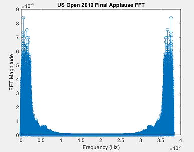
Final applause:

 

​

​

 

 

 

 

 

 

 

 

 

 

 

 

 

 

 

 

 

​

 

 

 

To get another audio clip to double check our findings from our original audio clip from Wimbledon, we selected a clip from a recent match at the US Open.  A couple things are evident from an initial listen and quick comparison between the two clips.  Everything seems to be louder at the US Open, apart from the ball hitting the rackets.  The crowds appear to cheer louder and more often than the fans at Wimbledon, the announcers for the US Open seem to speak louder into their microphones on the broadcast of the game, and in this specific match we chose, one of the players, Rafael Nadal, is famous for grunting as he hits the ball.

​

This quirky fact is visible when plotting the audio clip of Nadal hitting a ball.  The hit is the same, a delta-like auditory spike, but there is a horizontal cone that tapers down to the ambient volume immediately after Nadal hits the ball.  Since this sensation is actually quite similar to the pattern of noises a crowd makes and Nadal often-times makes the same noise, it shouldn’t be hard to filter out when our filter is designed to filter out those sorts of noises. The challenge will just be to manipulate the audio with a number of DSP tools that we have learned thus far and output an audio signal that has less noise and is easier to analyze.

 

​

Challenges

​

There are a couple of challenges that we have run into while working on the project. The first is the problem of distinguishing between the audio signals sent by the audience and the audio signals produced by the ball hitting the racket. Although the plot of the overall sound wave shows distinct differences between the two, with the former lasting much longer and having a slow decay and the latter resembling the Dirac delta function, the problem of filtering one of them out is more difficult than expected. A simple high pass filter did not quite accomplish the task as we had hoped. Although the ball audio generally has high frequency, the filter leaves in much of the player sounds, as well as does nothing to remove the noise, which is high frequency. Possible solutions to this problem include trying other types of high pass filters and designing a filter that magnifies large amplitudes to eliminate the noise. 

 

The other challenge is that this project is relatively obscure and unexplored. The main source of information for this project specifically is the IEEE article on this problem. The article lays out a useful foundation for the problem by breaking the tennis game up into   a block diagram of smaller chronological events. However, much of the work done on connecting the intermediate parts uses high level ideas from machine learning which would be difficult to incorporate into our project. Possible solutions to this include closely examining one of the intermediate paths at sufficient depth to be able to use it, and researching more general techniques for signal processing and auditory signal processing.

​

​

Next Steps

 

Some tasks we need to complete in the future include:

​

1. Finalize a method (or methods) for distinguishing between the sounds of the ball hitting the racquet and the player/ump/audience sounds. Also, evaluate the accuracy of this method by applying it to some game audio and manually checking the results.

​

2. Write an algorithm that, given an audio signal of a game, marks out the points in the time domain where the ball is being hit and the player, umpire, or audience are making noise. This will be using the methods from step 1.

​

3. Explore how the points in time of the ball hit noises and player/ump/audience noises indicate the game points. More specifically, develop an algorithm which takes in the points in time of the aforementioned audio cues and outputs a guess for the points in time of the game points. The accuracy of this algorithm can be evaluated through manually checking the game points.

 

​

Acquired Knowledge

​

A DSP tool that we utilized was actually a rather simple tool, the high pass filter. We desired to isolate just the sound of the ball, which has a normally high frequency, and the high pass would theoretically do just that. For this reason the use of filters and audio manipulation to single out noises such as the sharp pop of a ball being hit is vital to our assignment. Along the way we have learned that a simple high pass filter didn’t exactly do the job that we wanted it to, some extra noise was passing through the filter that wasn’t desirable. Although this is a minor setback, this works as a learning opportunity to experiment with different filters and parameters and develop a deeper understanding of the DSP tools. As we continue working on this project and analyzing the audio from tennis matches, it is clear that we will have many more opportunities to learn about filtering and audio signals.